Theoretical Motivations for Deep Learning

This post is based on the lecture “Deep Learning: Theoretical Motivations” given by Dr. Yoshua Bengio at Deep Learning Summer School, Montreal 2015. I highly recommend the lecture for a deeper understanding of the topic.

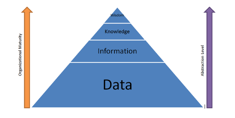
Deep learning is a branch of machine learning algorithms based on learning multiple levels of representation. The multiple levels of representation corresponds to multiple levels of abstraction. This post explores the idea that if we can successfully learn multiple levels of representation then we can generalize well.

The below flow charts illustrate how the different parts of an AI system relate to each other within different AI disciplines. The shaded boxes indicate components that are able to learn from data.

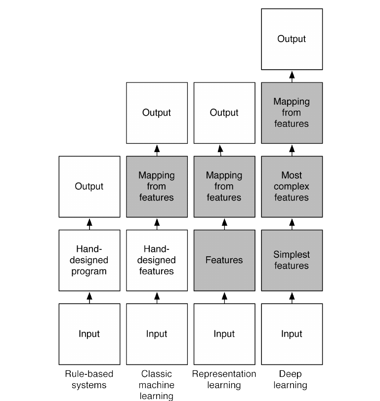
Rule-Based Systems

Rule-based systems are hand-designed AI programs. The knowledge required by these programs are provided by experts in the concerned field. That is why these systems are also called expert systems. These hand-designed programs contains facts and the logic to combine the facts to answer questions.

Classical Machine Learning

In classical machine learning, the important features of the input are manually designed and the system automatically learns to map the features to outputs. This kind of machine learning is used and works well for simple pattern recognition problems. It is well known that in practice most of the time is spent designing the optimal features for the system. Once the features are hand-designed, a generic classifier is used to obtain the output.

Representation Learning

Representation learning goes one step further and eliminates the need to hand-design the features. The important features are automatically discovered from data. In neural networks, the features are automatically learned from raw data.

Deep Learning

Deep learning is a kind of representation learning in which there are multiple levels of features. These features are automatically discovered and they are composed together in the various levels to produce the output. Each level represents abstract features that are discovered from the features represented in the previous level. Hence, the level of abstraction increases with each level. This type of learning enables discovering and representing higher-level abstractions. In neural networks, the multiple layers corresponds to multiple levels of features. These multiple layers compose the features to produce output.

Path to AI

The 3 key ingredients for ML towards AI:

1. Lots of Data

An AI system needs lots of knowledge. This knowledge either comes from humans who put it in or from data. In case of machine learning, the knowledge comes from data. A machine learning system needs lots and lots of data to be able to make good decisions. Modern applications of machine learning deals with data in form of videos, images, audio, etc which are complicated and require lots of data to learn from.

2. Very Flexible Models

The data alone is not enough. We need to translate the knowledge into something useful. Also, we have to store the knowledge somewhere. The models needs to be big and flexible enough to be able to do this.

3. Powerful Priors

Powerful priors are required to defeat the curse of dimensionality. Good priors induce fairly general knowledge about the world into the system.

Classical non-parametric algorithms can handle lots of data and are flexible models. However, they use the smoothness prior and that is not enough. Hereby, this post mostly deals with the third ingredient.

How do we get AI?

Knowledge

The world is very complicated and an AI has to understand it. It would require a lot of knowledge to reach the level of understanding of the world that humans have. An AI needs to have a lot more knowledge than what is being made available to the machine learning systems today.

Learning

Learning is necessary to acquire the kind of complex knowledge needed for AI. Learning algorithms involve two things - priors and optimization techniques.

Generalization

The aspect of generalization is central to machine learning. Generalization is a guess as to which configuration is most likely. A geometric interpretation is that we are guessing where the probability mass is concentrated.

Ways to fight the curse of dimensionality

The curse of dimensionality arises from high dimensional variables. There are so many dimensions and each dimension can take on lots of values. Even in 2 dimensions, the no of possible configurations is huge. It looks almost impossible to handle the possible configurations in higher dimensions.

Disentangling the underlying explanatory factors

An AI needs to figure out how the data was generated - the explanatory factors or the causes of what it observes. This is what science is trying to do - conduct experiments and come up with theories to explain the world. Deep learning is a step in that direction.

Why not classical non-parametric algorithms?

There are different definitions for the term non-parametric. We say that a learning algorithm is non-parametric if the complexity of the functions it can learn is allowed to grow as the amount of training data is increased. In other words, it means that the parameter vector is not fixed. Depending on the data we have, we can choose a family of functions that are more or less flexible. In case of a linear classifier - even if we get 10 times more data than what we already have, we are stuck with the same model. In contrast, for neural networks we get to choose more hidden units. Non-parametric is not about having no parameters. It’s about not having a fixed parameter. It’s about choosing the amount of parameters based on the richness of data.

The Curse of Dimensionality

The curse of dimensionality arises because of the many possible configurations in high dimensions. The number of possible configurations increases exponentially with the number of dimensions. Then, how can we possibly generalize to new configuration we have never seen? that is what machine learning is about.

The classical approach in non-parametric statistics is to rely on smoothness. It works fine in small dimensions but in high dimensions the average value either ends up with no examples or all examples in it. This is useless. To generalize locally, we need representative examples for all relevant variations. It is not possible to average locally and obtain something meaningful.

If we dig deeper mathematically, it’s not the number of dimensions but the number of variations of functions that we learn. In this case, smoothness is about how many ups and downs are present in the curve.

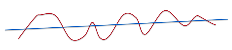
A line is very smooth. A curve with some ups and downs is less smooth but still smooth.

The functions we are trying to learn are very non-smooth. In case of modern machine learning applications like computer vision or natural language processing, the target function is very complex.

Many non-parametric statistics rely on something like gaussian kernel to average the values in some neighbourhood. However, Gaussian kernel machines need at least k examples to learn a function that has 2k zero-crossings along some line. The number of ups and downs could be exponential in the number of dimensions. It is possible to have a very non-smooth function even in 1-dimension.

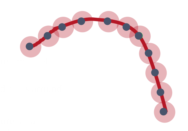
In a geometric sense, we have to put the probability mass where the structure is plausible. In the empirical distribution, the mass is concentrated at the training examples. Consider the above visualization with some 2-dimensional data points. In the smoothness assumption, the mass is spread around the the examples. The balls in the figure illustrate the gaussian kernels around each example. This is what many non-parametric statistical methods do. The idea seems plausible in this 2-dimensional case. However in higher dimensions, the balls will be so large that they cover everything or leave holes in places where there should be a high probability. Hence, the smoothness assumption is insufficient and we have to discover something smarter about the data - some structure. The figure depicts such a structure, a 1-dimensional manifold where the probability mass is concentrated. If we are able to discover a representation of the probability concentration, then we can solve our problems. The representation can be a lower dimensional one or along a different axis in the same dimension. We take a complicated and non-linear manifold and ‘flatten’ the manifold by changing the representation ie., we transform complicated distributions to a euclidean space. It is easy to make predictions, interpolation, density estimation, etc. in this euclidean space.

Bypassing the Curse

Smoothness has been the ingredient in most statistical non-parametric methods and it is quite clear that we cannot defeat the curse of dimensionality if we only use smoothness. We want to be non-parametric in the sense that we want the family of functions to grow in flexibility as we get more data. In neural networks, we change the number of hidden units depending on the amount of data.

We need to build compositionality into our ML models. Natural languages exploit compositionality to give representations and meanings to complex ideas. Exploiting compositionality gives an exponential gain in representational power. In deep learning, we use two priors:

1. Distributed Representations
2. Deep Architecture

Here, we make a simple assumption that the data we are observing came up by composition of pieces. The composition maybe be parallel or sequential. Parallel composition gives us the idea of distributed representations. It is basically the same idea of feature learning. Sequential composition deals with multiple levels of feature learning. An additional prior is that compositionality is useful to describe the world around us efficiently.

The Power of Distributed Representations

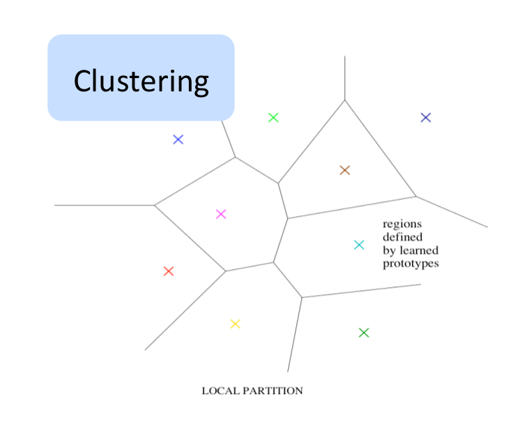
Non-distributed representations

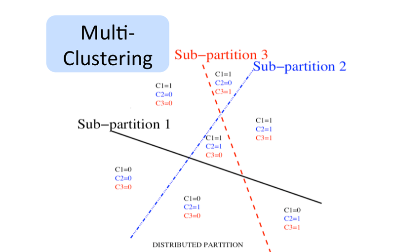
The methods that don’t use distributed representation are clustering, n-grams, nearest neighbours, RBF SVMs, decision trees etc. On a high level, these algorithms take the input space and split it into regions. Some algorithms have hard partitions while others have soft partitions that allow smooth interpolations between the nearby regions. There are different set of parameters for each region. The corresponding answer of each region and where the regions should be are tuned using the data. There is a notion of complexity tied to the number of regions. In terms of learning theory, generalization depends on the relationship between the number of examples needed and the complexity. A rich function requires more regions and more data. There is a linear relation between the number of distinguishable regions and the number of parameters. Equivalently, there is a linear relation between the number of distinguishable regions and number of training examples.

Why Distributed Representations?

There is another option. With distributed representations, it is possible to represent exponential number of regions with a linear number of parameters. The magic of distributed representation is that it can learn a very complicated function(with many ups and downs) with a low number of examples. In non-distributed representations, the number of parameters are linear to the number of regions. Here, the number of regions potentially grow exponentially with the number of parameters and number of examples. In distributed representations, the features are individually meaningful. They remain meaningful despite what the other features are. There maybe some interactions but most features are learned independent of each other. We don’t need to see all configurations to make a meaningful statement. Non-mutually exclusive features create a combinatorially large set of distinguishable configurations. There is an exponential advantage even if there is only one layer. The number of examples might be exponentially smaller for this prior. However, this is not observed in practice - there is a big advantage but not an exponential one. If the representations are good, then what it’s really doing is unfolding the manifold to a new flat coordinate system. Neural networks are really good at learning representations that capture the semantic aspects. The generalization comes from these representations. In classical non-parametric, we are not able to say anything about an example located in input space with no data. Whereas, with this approach we are able to say something meaningful about what we have not seen before. That is the essence of generalization.

Classical Symbolic AI vs Representation Learning

Distributed representations are at the heart of the renewal of neural networks in 1980’s - called connectionism or the connectionist approach. The classical AI approach is based on the notion of symbols. In symbolic processing of things like language or logic and rules, each concept is associated with a pure entity - a symbol. A symbol either exists or it doesn’t. There is nothing intrinsic that describes any relationship between them. Consider, the concept of a cat and a dog. In symbolic AI, they are different symbols with no relation between the them. In distributed representation, they share some features like being a pet, having 4 legs, etc. It makes more sense when thinking about concepts as patterns of features or patterns of activations of neurons in the brain.

Distributed Representations in NLP

There has been some interesting results in natural language processing with the use of distributed representations. I highly recommend the article Deep Learning, NLP, and Representations for a detailed understanding of these results.

The Power of Deep Representations

There is a lot of misunderstanding about what depth means. Depth was not studied before this century because people thought there was no need of deep neural networks. A shallow neural network with a single layer of hidden units is sufficient to represent any function with required degree of accuracy. This called the universal approximation property. But, it doesn’t tell us how many units is required. With a deep neural network we can represent the same function as that of a shallow neural network but more cheaply ie., with less number of hidden units. The number of units needed can be exponentially larger for a shallow network compared to a network that is deep enough. If we are trying to learn a function that is deep(there are many levels of composition), then the neural network needs more layers.

Depth is not necessary to have a flexible family of functions. Deeper networks does not correspond to a higher capacity. Deeper doesn’t mean we can represent more functions. If the function we are trying to learn has a particular characteristic obtained through composition of many operations, then it is much better to approximate these functions with a deep neural network.

Shallow and Deep computer program

“Shallow” computer program

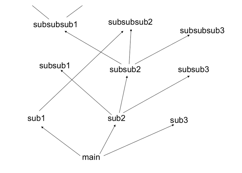“Deep” computer program

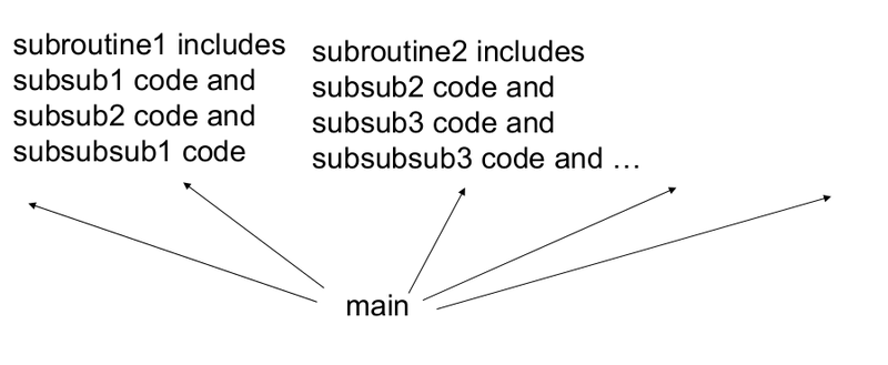
When writing computer programs, we don’t usually write the main program one line after another. Typically, we have subroutines that are reused. It is plausible to think that what the hidden units are doing as kind of subroutines for the bigger program that is at the final layer. Another way to think is that result of computation of each line in the program is changing the state of the machine to provide an input for the next line. The input at each line is the state of the machine and the output is a new state of the machine. This corresponds with a turing machine. The number of steps that a turing machine executes actually corresponds to the depth of computation. In principle, we can represent any function in two steps(lookup table). This doesn’t mean it will be able to compute anything interesting with efficiency. The kernel SVM or a shallow neural network can be considered as a kind of a lookup table. So, we need deeper programs.

Sharing components

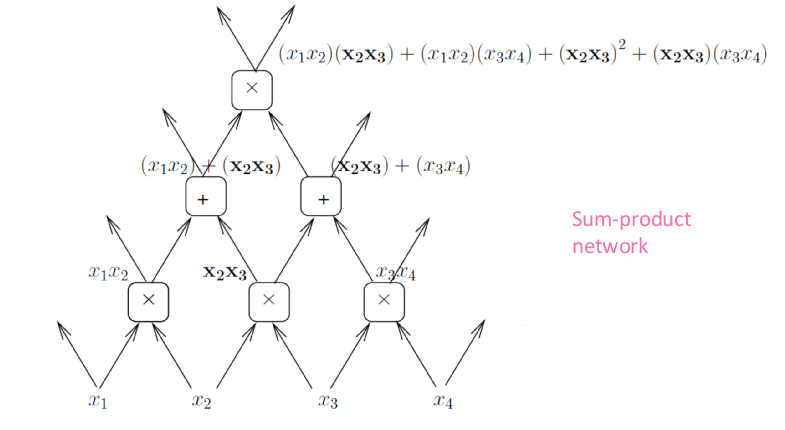
Polynomials are usually represented as a sum of products. Another way to represent polynomials is using a graph of computations where each node performs an addition or a multiplication. This way we can represent deep computations. Here, the number of computations will be smaller because we can reuse some operations.

There is new theoretical result that deeper nets with rectifier/maxout units are exponentially more expressive than shallow ones because they can split the input space in many more linear regions, with constraints.

The Mirage of Convexity

One of the reasons neural networks were discarded in the late 90’s is that the optimization problem is non-convex. We know from the late 80’s and 90’s that there are an exponential number of local minima in neural networks. This knowledge combined with the success of kernel machines in mid 90’s played a role in greatly reducing the interest of many researchers in neural networks. They believed that since the optimization is non-convex, there is no guarantee that we are going to find the optimal solution. Further, the network may get stuck on poor solutions. Something changed very recently over the last year. Now we have the theoretical and empirical evidence that the issue of non-convexity may not be issue at all. This changes the picture of what we have with optimization problem of neural networks.

Saddle Points

Let us consider the optimization problem in low dimensions vs high dimensions. In low dimensions, it is true that there exists lots of local minima. However in high dimensions, local minima are not really the critical points that are the most prevalent in points of interest. When we optimize neural networks or any high dimensional function, for most of the trajectory we optimize, the critical points(the points where the derivative is zero or close to zero) are saddle points. Saddle points unlike local minima, are easily escapable.

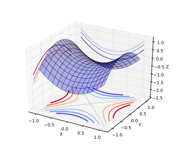
A saddle point is illustrated in the image above. In a global or local minima, all the directions are going up and in a global or local maxima, all the directions are going down. In case of local minima in a very high dimensional space(the space of parameters), all the directions should go up in all dimensions. If there is somehow a randomness in how all the functions are constructed and if the direction are independently chosen, it is exponentially unlikely that all directions go up except near the bottom of the landscape ie., near the global minima. The intuition is that when there is a minima that’s close to the global minima, all directions go up and it’s not possible to go further down. Hence, the local minima exists but are very close to global minima in terms of objective functions. Theoretical results from statistical physics and matrix theory suggests that for some families of functions that are fairly large, there is a concentration of probability between the index of the critical points and the objective function. Index is the fraction of directions that are going down. When index = 0, it is a local minimum and when index = 1, it is a local maximum. If index is something in between, then it is a saddle point. So, local minima is a special case of saddle point when index = 0. For a particular training objective, most of the critical points are saddle points with a particular index. Empirical results verify that indeed there is a tight relation between index and the objective function. It’s only an empirical validation and there is no proof that the results apply to optimization of neural networks. There is some evidence that the behaviour observed corresponds to what the theory suggests. In practice, it is observed that stochastic gradient descent will almost always escape from surfaces other than local minima.

Related papers:

1. On the saddle point problem for non‐convex optimization - Pascanu, Dauphin, Ganguli, Bengio, arXiv May 2014
2. Identifying and attacking the saddle point problem in high-­dimensional non-­convex optimization - Dauphin, Pascanu, Gulcehre, Cho, Ganguli, Bengio, NIPS 2014
3. The Loss Surface of Multilayer Nets - Choromanska, Henaff, Mathieu, Ben Arous & LeCun 2014

Other Priors That Work with Deep Distributed Representations

The Human Way

Humans are capable of generalizing form very few examples. Children usually learn new tasks from very few examples. Sometimes even from one example. Statistically, it is impossible to generalize from one example. One possibility is that the child is using knowledge from previous learning. The previous knowledge can be used to build representations such that in the new representation space it is possible to generalize from a single example. Thus, we need to introduce more priors than distributed representations and depth.

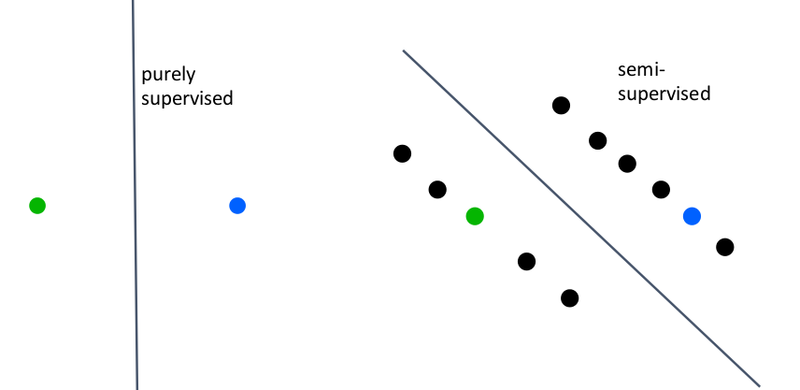
Semi-Supervised Learning

Semi-supervised learning falls between unsupervised learning and supervised learning. In supervised learning, we use only the labelled examples. In semi-supervised learning, we also make use of any unlabelled examples available. The image below illustrates how semi-supervised learning may find a better boundary of separation with use unlabelled examples.

Multi-Task Learning

Generalizing better to new tasks is crucial to approach AI. Here, the prior is the shared underlying explanatory factors between tasks. Deep architectures learn good intermediate representations that can be shared across tasks. Good representations that disentangle underlying factors of variation make sense for many tasks because each task concerns a subset of the factors.

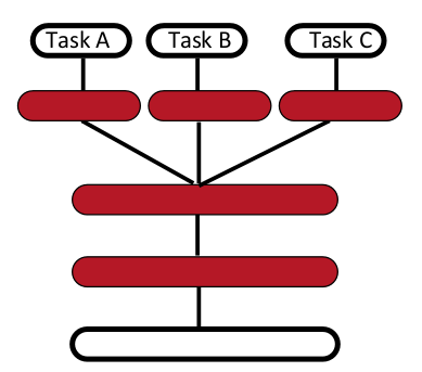
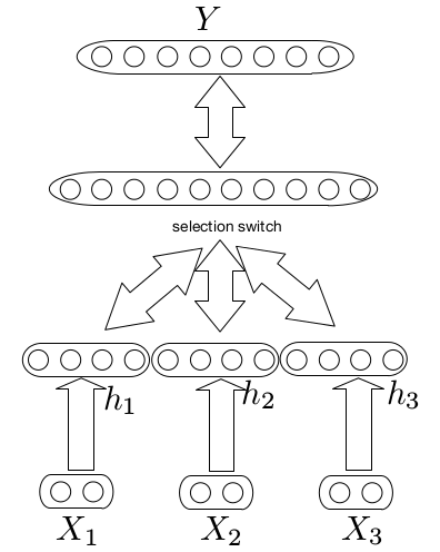
The following figure illustrates multi-task learning with different inputs,

Learning Multiple Levels of Abstraction

The big payoff of deep learning is to allow learning higher levels of abstraction. Higher-level abstractions disentangle the factor of variation, which allows much easier generalization and transfer.

Conclusion

• Distributed representation and deep composition are priors that can buy exponential gain in generalization.
• Both these priors yield non-local generalization.
• There is strong evidence that local minima are not an issue because of saddle points.
• We have to introduce other priors like semi-supervised learning and multi-task learning that work with deep distributed representations for better generalization.